Forecasting is a statistical technique used to make predictions about future value(s) of a quantity based on past known values. Common applications of forecasting can be found in weather forecasts, sales planning and production planning.
Definitions
In the context of forecasting, the quantity being forecasted is
usually referred to as the observable, the future
values predicted by the process as the forecast,
the past data used to generate the forecast as the
observations (or the sample), and
an individual observation value as a data point.
For the rest of this post, we will use the data points
[1125, 1177, 1224, 1264, 1326, 1367, 1409, 1456, 1500, 1570, 1636, 1710, 1440, 1493, 1553, 1611, 1674, 1742, 1798, 1876, 1955, 2033, 2115, 2190, 1955, 2022, 2117, 2216, 2295, 2403, 2498, 2602, 2723, 2837, 2948, 3066]
collected for some arbitrary quantity as an example.
The following image depicts these data points graphically.
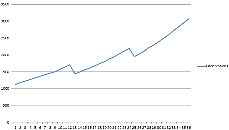
Figure 1: Example observations
It is common for forecasting techniques to make predictions corresponding to at least some, if not all of the (past) observed data points (in addition to generating predictions for the future). This allows the forecast to be compared with the (actual) observations to understand forecast accuracy.
A common measure for forecast accuracy is the difference between
a data point and its corresponding prediction, known as the
error (that is,
error = observation - prediction).
If a prediction is higher than the data
point (prediction > observation), the error is
negative, if both are the same
(prediction = observation),
the error is zero, and if the prediction is lower
than the data point (prediction < observation),
the error is positive. Given that the error can be negative,
zero or positive, it is more common to use the square of the
error, known as the squared-error, which is
always zero or positive. This is done to avoid situations where
negative errors cancel out positive errors exactly, thereby
providing a false sense of forecast accuracy.
Forecasts for the same observations, generated using different forecasting techniques can be compared to each other by comparing the squared-errors (or just the errors, although this is usually avoided) for the different forecasts. Lower the squared-error, higher the accuracy of the associated forecasting technique.
Forecasting basics
For most observations, there are three important points of
interest. The first, known as the level is just
the simple average of all data points. The image below shows
the observations introduced earlier, with their level.
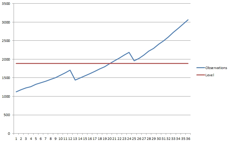
Figure 2: Example observations, with level
The second, known as the trend indicates whether
the observations increase or decrease on an overall basis
(from the first to the last data point). A visual inspection of
the example observations above shows that they have a
(significant) increasing trend.
The third and last point of interest is the
seasonality, which is defined as the periodicity
of any patterns embedded within the observations. The example
observations above have a periodicity of 12, as
there is an upward trend for 12 data points, followed by a
downward trend for 1 data point, followed by a repetition of
the pattern.
Simple Exponential Smoothing
It is generally seen that more the number of data points used to generate a forecast, higher the forecast accuracy. This is because such a forecast would have an "insight" into a larger number of data points, thereby being able to assess the level, trend and seasonality to a greater accuracy. However, it is reasonable to expect that more recent data points should have a higher contribution towards a prediction than older ones, since more recent events are more likely to influence the future.
Exponential smoothing is a class of forecasting techniques that use the weighted average method for generating the forecast. These techniques use progressively decreasing weights for older observations to let more recent data points have higher influence on the forecast, and older ones to have lower influence.
The simplest of these techniques, aptly called
Simple Exponential Smoothing (or
Single Exponential Smoothing) uses a single parameter
to assign "exponentially" lower weights to older data points.
A smooth version is generated for each data point.
If there are \(\bf n\) observations, denoted by
\(\bf O_1, O_2, ..., O_n\), their smooth versions are calculated
as:
\(S_i = \alpha{O_{i-1}} + (1 - \alpha)S_{i-1}\), or alternatively as
\(S_i = S_{i-1} + \alpha(O_{i-1} - S_{i-1})\)
where, \(\bf i\) ranges from \(\bf 2\) to \(\bf n\), \(\alpha\)
is called the smoothing parameter, and \(\bf S_i\)
are the smooth versions of the observations \(\bf O_i\). There
is no smooth version \(\bf S_1\) for the first observation
\(\bf O_1\). The value of \(\alpha\) ranges between \(0\) and
\(1\).
a. Effect of the smoothing parameter
When \(\alpha = 0\), \(1 - \alpha = 1\), and the formula for calculating the smooth versions becomes \(S_i = S_{i-1}\), that is, each forecast value is the same and has no dependence on the observations. Consequently, the forecast has no predictive value at all (since each predicted value is the same).
Similarly, when \(\alpha = 1\), \(1 - \alpha = 0\), and the formula becomes \(S_i = O_{i-1}\), that is, each forecast value is the same as the previous observation. Consequently, this too has no preditive value at all.
For these reasons, neither \(0\), nor \(1\) is a good value for \(\alpha\).
The quantity mean squared error (MSE) is calculated
as the simple average of the squared errors, that is:
\(MSE = \frac{1}{n}[(O_2 - S_2)^2 + (O_3 - S_3)^2 + ... + (O_n - S_n)^2]\)
MSE is a measure of the forecast accuracy. Lower the MSE, more accurate the forecast, and vice versa. Therefore, in real-world scenarios, the value of \(\alpha\) is chosen such that the MSE is minimized.
b. Finding optimal \(\alpha\)
The optimal value of \(\alpha\) can be determined through trial-and-error, beginning with some value for the smoothing parameter between \(0\) and \(1\). The MSE can then be calculated by varying the value of the smoothing parameter by small amounts and comparing it with the previous value to see if it decreases or increases.
The trial-and-error method can be quite time-consuming if the observations fluctuate too much and if the value of \(\alpha\) is required to a high degree of accuracy, say, up to a certain number of decimal places. It is therefore commonplace to use an optimization method to find the optimal value for \(\alpha\). One such method is the Levenberg-Marquardt (LM) method.
The LM method relies upon finding the Jacobian of a function at every point to determine if the search for the optimal parameter value is progressing in the right direction. The Jacobian for a function \(S\) of \(k\) parameters \(x_k\) is a matrix, where an element \(J_{ik}\) of the matrix is given by \(J_{ik} = \frac{\partial S_i}{\partial x_k}\), \(x_k\) are the \(k\) parameters on which the function \(S\) is dependent, and \(S_i\) are the values of the function \(S\) at \(i\) distinct points.
In the case of simple exponential smoothing, there is only one parameter \(\alpha\) that impacts the predicted value for a given observed value. Therefore, the Jacobian (\(J\)) depends on only this one parameter \(\alpha\) and thereby reduces to \(J_i = \frac{\partial S_i}{\partial \alpha}\), or
\(J = \begin{bmatrix}J_2 & J_3 & ... & J_n \end{bmatrix} = \begin{bmatrix}\frac{\partial S_2}{\partial \alpha} & \frac{\partial S_3}{\partial \alpha} & ... & \frac{\partial S_n}{\partial \alpha} \end{bmatrix}\)
Given that the function \(S\) is defined for simple exponential smoothing as \(S_i = S_{i-1} + \alpha(O_{i-1} - S_{i-1})\) (see above),
\(J_i = \frac{\partial S_i}{\partial \alpha}\) becomes
\(J_i = \frac{\partial (S_{i-1} + \alpha(O_{i-1} - S_{i-1}))}{\partial \alpha}\), or
(by the associative rule of differentiation)
\(J_i = \frac{\partial S_{i-1}}{\partial \alpha}
+ \frac{\partial (\alpha(O_{i-1}
- S_{i-1}))}{\partial \alpha}\), or
(by the associative rule of differentiation)
\(J_i = \frac{\partial S_{i-1}}{\partial \alpha}
+ \frac{\partial (\alpha{O_{i-1}})}{\partial \alpha}
- \frac{\partial (\alpha{S_{i-1}})}{\partial \alpha}\), or
(by the chain rule of differentiation)
\(J_i = \frac{\partial S_{i-1}}{\partial \alpha}
+ \alpha{\frac{\partial O_{i-1}}{\partial \alpha}}
+ O_{i-1}{\frac{\partial \alpha}{\partial \alpha}}
- \alpha{\frac{\partial S_{i-1}}{\partial \alpha}}
- S_{i-1}{\frac{\partial \alpha}{\partial \alpha}}\), or
(upon simplification)
\(J_i = \frac{\partial S_{i-1}}{\partial \alpha}
+ O_{i-1}
- \alpha{\frac{\partial S_{i-1}}{\partial \alpha}}
- S_{i-1}\)
(since \(\frac{\partial O_{i-1}}{\partial \alpha} = 0\), given that
\(O_{i-1}\) does not depend on \(\alpha\)), or
(upon rearrangement of terms)
\(J_i = O_{i-1} - S_{i-1} + (1 - \alpha)\frac{\partial S_{i-1}}{\partial \alpha}\), or
using the fact that \(\frac{\partial S_{i-1}}{\partial \alpha} = J_{i-1}\)
\(J_i = O_{i-1} - S_{i-1} + (1 - \alpha)J_{i-1}\)
Since \(S_2 = O_1\), \(J_2 = \frac{\partial S_2}{\partial \alpha} = 0\). This gives an initial value for the Jacobian that can be used to derive the rest using the recursive formula derived above, for any given value of \(\alpha\), that is
\(J_2 = 0\)
\(J_3 = O_2 - S_2 + (1-\alpha)J_2\)
\(J_4 = O_3 - S_3 + (1-\alpha)J_3\)
\(J_5 = O_4 - S_4 + (1-\alpha)J_4\)
... and so on.
The Apache Commons Math library provides an excellent implementation of the LM method, should there be a need to write a software program for finding optimal \(\alpha\) for simple exponential smoothing.
For the example observations above, an optimal \(\alpha\) of
0.5522115480262714 is obtained. Using this value
yields the following forecast:
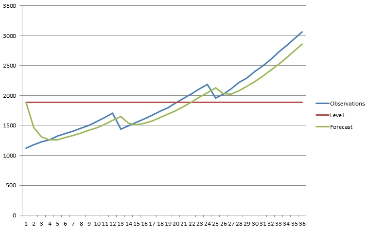
Figure 3: Example observations, with level and forecast
The following Java code shows how to use the Apache Commons Math library (version 3.6.1 to be precise) to find the optimal value for \(\alpha\) (Java 8 or higher required).
  /**
   * Optimizes the value for the smoothing factor for a set of
   * observations using the {@literal Levenberg-Marquardt (LM)} method,
   * which is a non-linear, least-squares, curve-fitting algorithm. This
   * method generates predictions for the given observations, starting
   * with an initial guess for the smoothing factor, and iteratively
   * changing the value of the smoothing factor until one is found that
   * minimizes the {@literal sum-squared-error (MSE)} for the given
   * observations.
   */
  public class LevenbergMarquardtOptimizer
  {
    /**
     * Finds the optimal value for the smoothing factor for a
     * collection of observations, such that the value can be used to
     * generate a forecast that is as close to the observations as possible.
     *
     * @param observations      The observations for which the optimal value of
     *                          the smoothing factor is required.
     * @return An optimal value for the smoothing factor for the given
     * observations.
     */
    public double optimize(final double[] observations)
    {
      return new LevenbergMarquardtOptimizer().optimize(optimizationModel(observations))
                                    .getPoint()
                                    .getEntry(0);
    }

    /**
     * Creates a baseline of a collection of observations. The baseline is
     * used to generate predictions for the observations, as well as fine-tune
     * the model to produce optimal predictions.
     *
     * @param observations A collection of observations.
     * @return A baseline version of the observations.
     */
    private double[] baselineObservations(final double[] observations)
    {
      final double[] baseline = new double[observations.length];

      System.arraycopy(observations, 0, baseline, 1, observations.length - 1);

      return baseline;
    }

    /**
     * Gets the simple average for a collection of observations. This is used
     * as the first prediction for the given observations.
     *
     * @param observations The observations for which the first prediction is
     *                     required.
     * @return The first prediction for the observations.
     */
    private double firstPrediction(final double[] observations)
    {
      return Arrays.stream(observations)
                    .boxed()
                    .mapToDouble(d -> d)
                    .average()
                    .orElse(0);
    }

    /**
     * Converts a collection of observations into a
     * {@literal least-squares curve-fitting problem} using an initial
     * value for the smoothing factor. The smoothing factor is used for
     * applying exponential smoothing so that the resultant problem can
     * be fed to a curve-fitting algorithm for finding the optimal value
     * of the smoothing factor .
     *
     * @param observations      The observations to convert to a least-squares
     *                          curve-fitting problem.
     * @return A {@link LeastSquaresProblem}.
     */
    private LeastSquaresProblem optimizationModel(final double[] observations)
    {
      return new LeastSquaresBuilder()
          .checkerPair(new SimpleVectorValueChecker(1e-6, 1e-6))
          .maxEvaluations(100)
          .maxIterations(100)
          .model(optimizationModelFunction(observations), optimizationModelJacobian(observations))
          .parameterValidator(alphaValidator())
          .target(observations)
          .start(new double[] { 0.5 })
          .build();
    }

    /**
     * Gets the model function to use for optimizing the value of
     * the smoothing factor, which is just the predicted value for
     * each observed value. The optimization algorithm then uses the
     * difference between the observed and corresponding predicted
     * values to find the optimal value for the smoothing factor.
     *
     * @param observations      The observations for which the optimal value of
     *                          the smoothing factor is required.
     * @return A {@link MultivariateVectorFunction}.
     */
    private MultivariateVectorFunction optimizationModelFunction(final double[] observations)
    {
      return params -> smoothenObservations(observations, params[0]);
    }

    /**
     * Gets the Jacobian (\(j\)) corresponding to the model function
     * used for optimizing the value of the smoothing factor.
     *
     * @param observations      The observations (\(y_t\)) for which the
     *                          optimal value of the smoothing factor is
     *                          required.
     * @return A {@link MultivariateMatrixFunction}, which is a
     * single-column matrix whose elements correspond to the
     * Jacobian of the model function.
     */
    private MultivariateMatrixFunction optimizationModelJacobian(final double[] observations)
    {
      return params -> {
        final double alpha = params[0];

        // Smoothen the observations.
        final double[] smoothed = smoothenObservations(observations, alpha);

        final double[][] jacobian = new double[observations.length][1];

        // Prepare a baseline for the observations.
        final double[] baseline = baselineObservations(observations);

        // The first element of the Jacobian is simply the first observation,
        // since there is no prior prediction for it.
        jacobian[0][0] = observations[0];

        // Calculate the rest of the Jacobian using the current observation
        // and the immediately previous prediction.
        for (int i = 1; i < jacobian.length; ++i)
        {
          jacobian[i][0] = baseline[i] - smoothed[i - 1]
              + Math.min(1, i - 1) * Math.pow(1 - alpha, i - 1) * jacobian[i - 1][0];
        }

        return jacobian;
      };
    }

    /**
     * Smoothens a collection of observations by dampening them exponentially
     * using a smoothing factor.
     *
     * @param observations The observations to smoothen.
     * @param alpha        The smoothing factor.
     * @return Smoothened observations.
     */
    private double[] smoothenObservations(final double[] observations, final double alpha)
    {
      final double[] smoothed = new double[observations.length];

      // Generate the first smooth observation using a specific strategy.
      smoothed[0] = firstPrediction(observations);

      // Prepare a baseline for the observations.
      final double[] baseline = baselineObservations(observations);

      // Generate the rest using the smoothing formula and using the baseline
      // values instead of the observations directly.
      for (int i = 1; i < observations.length; ++i)
      {
        smoothed[i] = smoothed[i - 1] + alpha * (baseline[i] - smoothed[i - 1]);
      }

      return smoothed;
    }
  }
Reference
An excellent overview of simple exponential smoothing can be found here.